Accessing data with odc-stac#

Introduction#

In this tutorial we will use Python libraries to find and load Land Use and Land Cover data from the freely available Impact Observatory Annual Land Use Land Cover product. After loading the data, we will export each year of data as a Cloud Optimised GeoTIFF. This will allow you to further view or work with the data in GIS software and other tools.

During the tutorial, we will:

Specify our search in terms of:
- what (data provider and product)
- where (area of interest)
- when (date range)
Use pystac-client to connect to a Spatio-Temporal Asset Catalog (STAC) endpoint and search for data matching our what, where, and when
Use odc-stac to load the matching data into memory
Visualise and export the data

There is no need to install anything. This tutorial runs in an online environment that we have prepared for you.

Launch tutorial environment#

Right-click on the Binder button below and select Open Link in New Window to launch the tutorial environment. This will allow you to keep the tutorial instructions open alongside the environment.

The tutorial environment may take a few minutes to start.

Once launched, you should see a Jupyter notebook environment with the tutorial notebook open. The tutorial notebook has headers that match up with the tutorial instructions on this page.

We also recommend that you open the file browser by clicking the folder icon on the left-hand menu bar (circled in purple in the top-left of the image above). This will allow you to see the output files at the end of the tutorial.

Note

For this tutorial, we believe you will learn more if you type the code yourself, rather than using copy-paste. Typing encourages you to slow down and think about what you’re doing, which will help you gain understanding!

If you are stuck at any point, open the tutorial_solution.ipynb notebook that is available in the file browser.

Tutorial#

Python imports#

The notebook requires five libraries to run:

geopandas for loading an area of interest from a GeoJSON file
odc.geo for exporting loaded data
odc.stac for loading data
planetary_computer to provide authentication when accessing data
pystac-client for querying catalogs of data

We will import either the library, or specific functions and classes from the library. Type the following into the empty cell below the Python imports heading:

import geopandas as gpd
from odc.geo.xr import write_cog
from odc.stac import load
import planetary_computer
from pystac_client import Client

When you have finished, run the cell by pressing Shift+Enter on your keyboard.

Set up query parameters#

In this section of the tutorial, you will specify:

The area you want to load data for
The date range you want to load data for
The data source you want to load from

Area of interest#

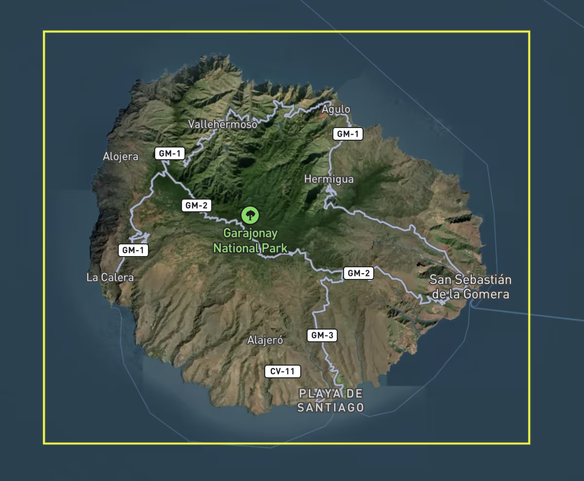
We specify the area of interest using the aoi.geojson file, which can be loaded with geopandas.

The area of interest is the island of La Gomera, one of the Canary Islands.

A map of La Gomera with satellite imagery, with the area of interest shown as a yellow bounding box.

Type the following into the empty cell below the Area of interest heading:

desired_aoi = gpd.read_file("aoi.geojson")
desired_aoi_geometry = desired_aoi.iloc[0].geometry

When you have finished, run the cell by pressing Shift+Enter on your keyboard.

Date range#

We must specify a start and end date for our query. Type the following into the empty cell below the Date range heading:

desired_start_date = "2017-01-01"
desired_end_date = "2023-01-01"
desired_date_range = (desired_start_date, desired_end_date)

When you have finished, run the cell by pressing Shift+Enter on your keyboard.

STAC metadata#

Many Earth observation data providers generate STAC metadata, which can be used to find and load data you’re interested in. STAC metadata has four important components:

Catalog: A structure for organising multiple datasets managed by a given provider. For example, Planetary Computer’s Catalog
Collection: A structure for organising all items in a single dataset. For example, Land Use Land Cover Collection
Item A single spatio-temporal item, such as one observation in a dataset. For example, Land Use Land Cover Data for Supercell 28R in 2023
Asset A single data measurement associated with an item, such as a single band. The Land Use Land Cover Dataset has only one asset, called “data”.

We must specify the URL for the catalog we want to search, along with the desired collection (io-lulc-annual-v02) and asset (data). The precise items that we need to load will be returned by a query that we run later.

Type the following into the empty cell below the STAC metadata heading:

catalog_url = "https://planetarycomputer.microsoft.com/api/stac/v1/"
desired_collections = ["io-lulc-annual-v02"]
desired_assets = ["data"]

When you have finished, run the cell by pressing Shift+Enter on your keyboard.

Connect to catalog and find items#

We use pystac_client.Client to connect to Planetary Computer’s STAC catalog. We also use planetary-computer’s sign_inplace modifier to authorise our connection. Type the following into the empty cell below the Connect to catalog and find items heading:

stac_client = Client.open(
   url=catalog_url,
   modifier=planetary_computer.sign_inplace,
)

When you have finished, run the cell by pressing Shift+Enter on your keyboard.

Search for items#

After setting up the Client, we use pystac_client.Client.search() to find items that match our chosen collection, area of interest, and date range. Type the following into the empty cell below the Search for items heading:

items = stac_client.search(
    collections=desired_collections,
    intersects=desired_aoi_geometry,
    datetime=desired_date_range,
).item_collection()

print(f"Found {len(items)} items")

When you have finished, run the cell by pressing Shift+Enter on your keyboard. After running the cell, you should see a printed sentence reporting “Found 7 items”

Troubleshooting#

If the sentence shows a different number of items, try checking whether your desired_date_range parameter is correct by printing it:

print(desired_date_range)

should return ('2017-01-01', '2023-01-01'). If you see a different date range, return to the Date range section and ensure your desired_start_date and desired_end_date values match those given in the instructions.

Load items with odc-stac#

After producing a list of items to load, we can use odc.stac.load() to read the requested assets from the items and return them as xarrays.

Type the following into the empty cell below the Load items with odc-stac heading:

ds = load(
   items=items,
   bands=desired_assets,
   geopolygon=aoi_geometry,
   crs="utm",
   resolution=30,
)

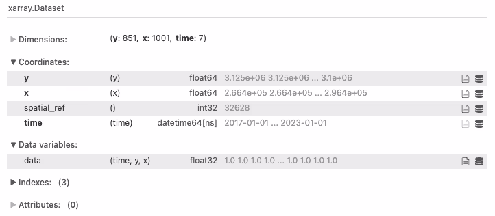
ds

When you have finished, run the cell by pressing Shift+Enter on your keyboard.

After running the cell, you should see an xarray.Dataset summary.

A table showing a summary of the loaded xarray, including dimensions, coordinates, and data variables.

Visualise loaded data#

To confirm that we have loaded the requested data, it is useful to visualise it. We can use the xarray plotting functionality to make a basic plot.

Type the following into the empty cell below the Visualise loaded data heading:

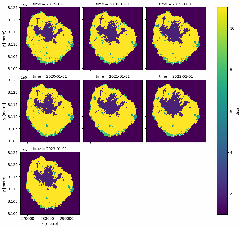
ds["data"].plot.imshow(col="time", col_wrap=3)

When you have finished, run the cell by pressing Shift+Enter on your keyboard. After running the cell, you should see the following visualisation. The colours in the plot represent the following land cover classes:

Colour	Land cover class
dark blue	water
green	built area
yellow	rangeland
mid blue	trees

A series of images showing the land cover data for each year, from 2017 to 2023. Each image shows the island in green, yellow and mid blue, surrounded by ocean in dark blue.

Advanced visualisation#

The code we’ve used provides us a visualisation that allows us to check that the data loaded successfully.

To produce a more descriptive plot, and understand the data, we recommend reviewing the io-lulc-annual-v02 example notebook that Microsoft Planetary Computer provide for this dataset.

Export loaded data#

Once you have loaded and checked your data, it is often useful to export it. This allows you to use the data in other software and analyses. We use odc.geo.xr.write_cog() to generate and write these files from an xarray.DataArray.

The code below extracts the year of each image from the dataset, then uses a loop to export each dataset to a new file.

Type the following into the empty cell below the Export loaded data heading:

years = ds.time.dt.strftime("%Y").values

for timestep in range(len(ds.time)):

    ds_single_year = ds["data"].isel(time=timestep)

    write_cog(
        ds_single_year,
        f"LULC_{years[timestep]}.tif",
        overwrite=True,
    )

When you have finished, run the cell by pressing Shift+Enter on your keyboard. You should see seven new files in the file browser, starting with LULC_2017.tif and ending with LULC_2023.tif.

Tutorial complete!#

Congratulations, you’ve used pystac-client to search for data in a public STAC catalog and odc-stac to load the data into an xarray.Dataset. In the last step, you exported the loaded data as a series of Cloud Optimised GeoTIFF files, which you can now use in other applications.

Note

Make sure you download these files from the file browser before exiting the tutorial space as they will be deleted when the tutorial space is closed.

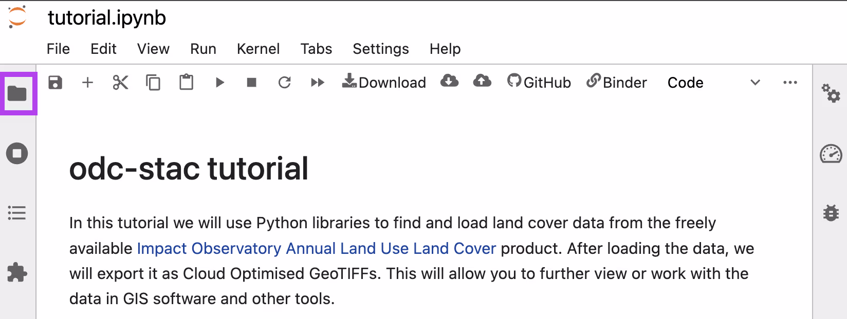
To download, open the file-browser by clicking the folder icon in the left menu bar. Then, download the Land Use Land Cover file for each year (denoted as LULC_year.tif) by right-clicking each file and selecting Download.